The Sacred Nine Spots

Quantifying and Optimising a Field Setting through data.

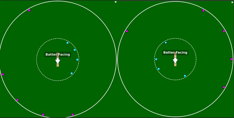
These are two field settings (worst and best) against Rohit Sharma on short-of-good-length deliveries from pacers. There's no prize for guessing which is which. The question is, how much better is the second one? Is there a way to quantify the expected runs saved? I have attempted this here in this piece. The answer is that the second field is expected to cover 73% of Rohit’s runs, compared to just 31% in the first case.

Field settings are just greedy optimizations. You have a fixed number of resources (nine fielders) to work with, and you are mostly looking to maximize the 'runs saved' variable. Defining the problem this way is the first step we can take toward solving field settings using data. Now that the problem is laid out, we move toward the solution. Since our focus is on run-saving, we will only consider the placement of fielders on the 30-yard and boundary circles. Positions like slips or gully are set aside for this analysis

Scoring Patterns and Runs Classes

The primary information we need to set a field against any batter is their scoring areas. I am using sectors of a circle here. Twenty-four 15-degree sectors are used. Each sector has an expected run value attached to it (calculated for each length against spin/pace). I also wanted to segregate based on line, but that led to data sparsity.

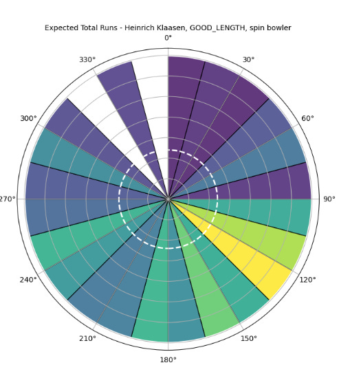
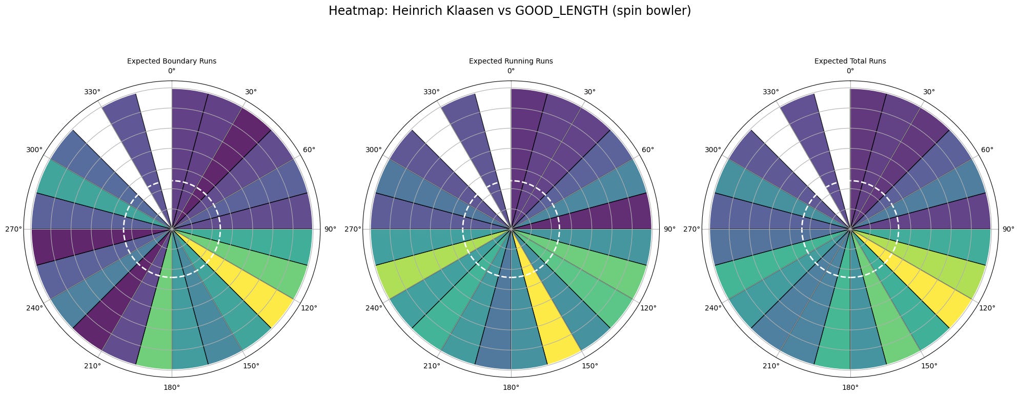
The plot indicates Klaasen’s effective pickup of good-length balls toward deep mid-wicket against spinners. But do we know from expected runs alone how those runs are scored? We will need information regarding the balance between scoring through boundaries and running between the wickets in each sector. Only then can we make decisions, such as whether a fielder is required on the ropes or if we can save an outfielder in that sector. This is achieved by dividing the runs into two classes: the boundary class and the running class. The idea is to know what expected runs could have been stopped by an infielder (running class). The classes are not mutually exclusive, however, because some boundaries—grounded fours—can also be covered by infielders. Due to a lack of data on aerial versus grounded shots, fours have been included with a weight factor of 0.5 in the running class. These are the final classes:

• Running: Ones, Twos, Threes, Grounded Fours

• Boundary: Fours and Sixes

Note that these classes are not disjoint; grounded fours are a common element.

The greedy algorithm thus maximises the following value -

This formula has an assumption: boundary fielders will not cover ones, twos, and threes. While it is not possible to know the extent to which these runs can be saved by outfielders without fielding data, we can determine what type of fielders we need in the outfield in different sectors. We will come back to this later.

Fielder and Field Restrictions

We now have the batter’s scoring pattern. But before we start placing fielders optimally, we need to know a few more conditions:

• Fielding Restrictions: Two outfielders in the Powerplay, five outfielders outside the Powerplay, a maximum of five fielders on the leg side, a maximum of two behind square leg, and no fielders in the umpire-wicketkeeper straight line.

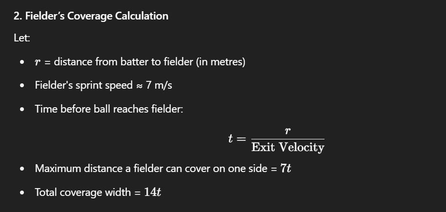
• Fielder Restrictions: Now, this is a part where good fielding data would have been of great help. What I wanted to know was an approximate angle coverage value (subtended at the center) that an average fielder is expected to cover. Due to the lack of such data, I had to dig for some values through which I could approximate this. This is the working:

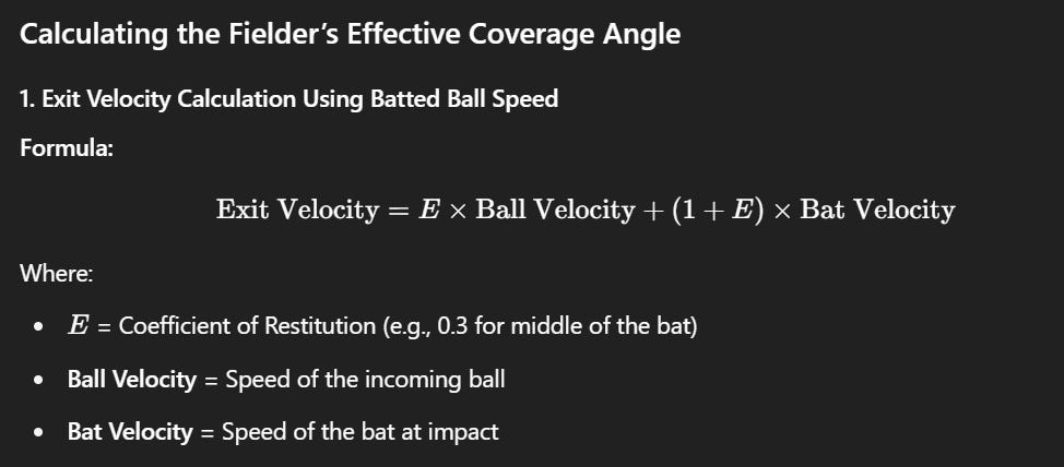
Refer - Batted Ball Speed for the formula and E value

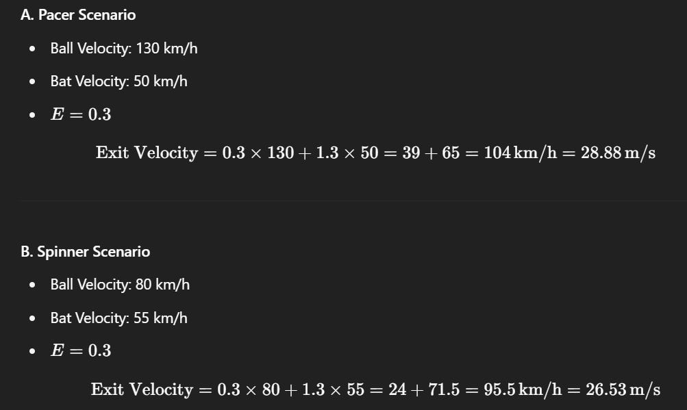
Bat Velocity Data - Grounded Boundary Shot at Top Level

Refer - Fielder Speed Data

(Thanks to Himanish Ganjoo for helping out here)

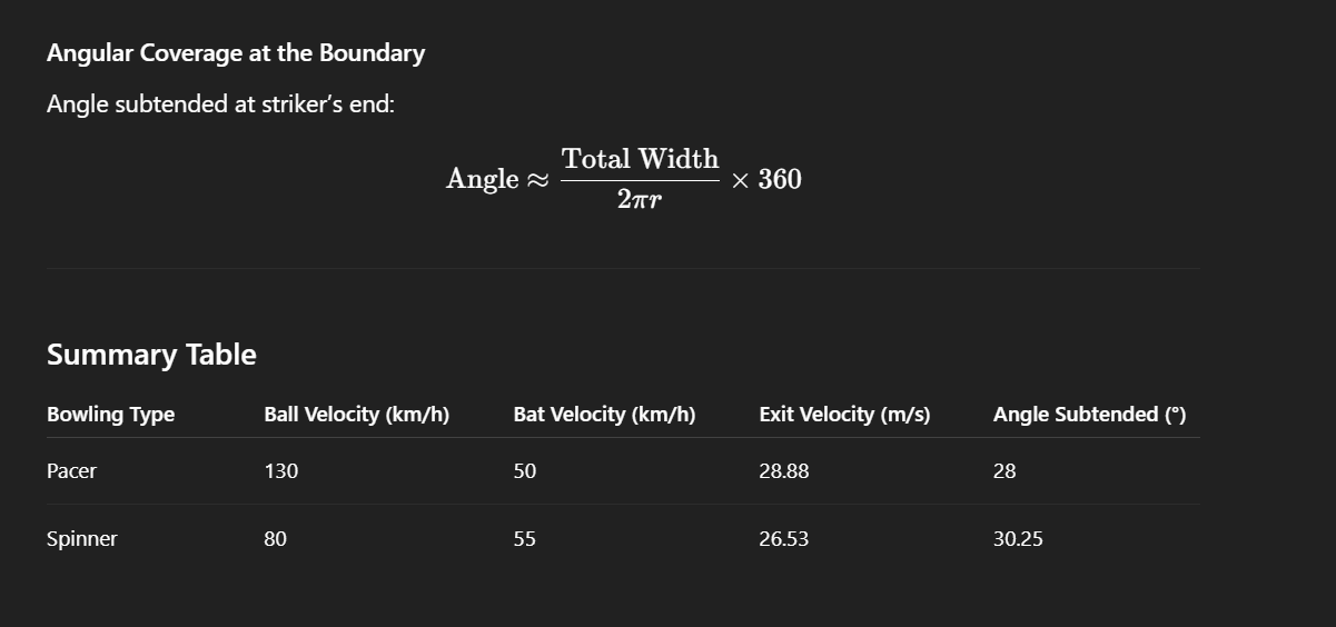
A 30 degree coverage angle thus seems acceptable for both pacers and spinners. This also gives us another restriction - A minimum of 30 degree gap between two fielders because overlaps would mean wastage of coverage area.

Greedy Setting and Using Protection Statistics

We are moving forward now with putting nine fielders greedily, keeping in mind the restrictions. I have used Dynamic Programming here. For an angle x moving from 0 to 360, number of outfielders - m moving from 0 to 5 (2 for powerplay), number of infielders - n moving from 0 to 4 (7 for powerplay). I compare three values -
1. Runs_Covered[x-1][m][n]
2. Runs_Covered[x-30][m-1][n] + Boundary Coverage of an outfielder at x
3. Runs_Covered[x-30][m][n-1] + Running Coverage of an infielder at x
And I go ahead with the maximum value. In words, I am checking whether its optimal to add a fielder at angle x (if yes, then infielder or outfielder?) or its better to skip. I subtract 30 for checking for fielder addition because of the minimum gap we discussed earlier. Finally the value at Runs_Covered[359][5/2][4/7] gives me the highest possible coverage.

Samson and the Cut Shot

We’ll try it out on a player now, I’m going with Sanju Samson -

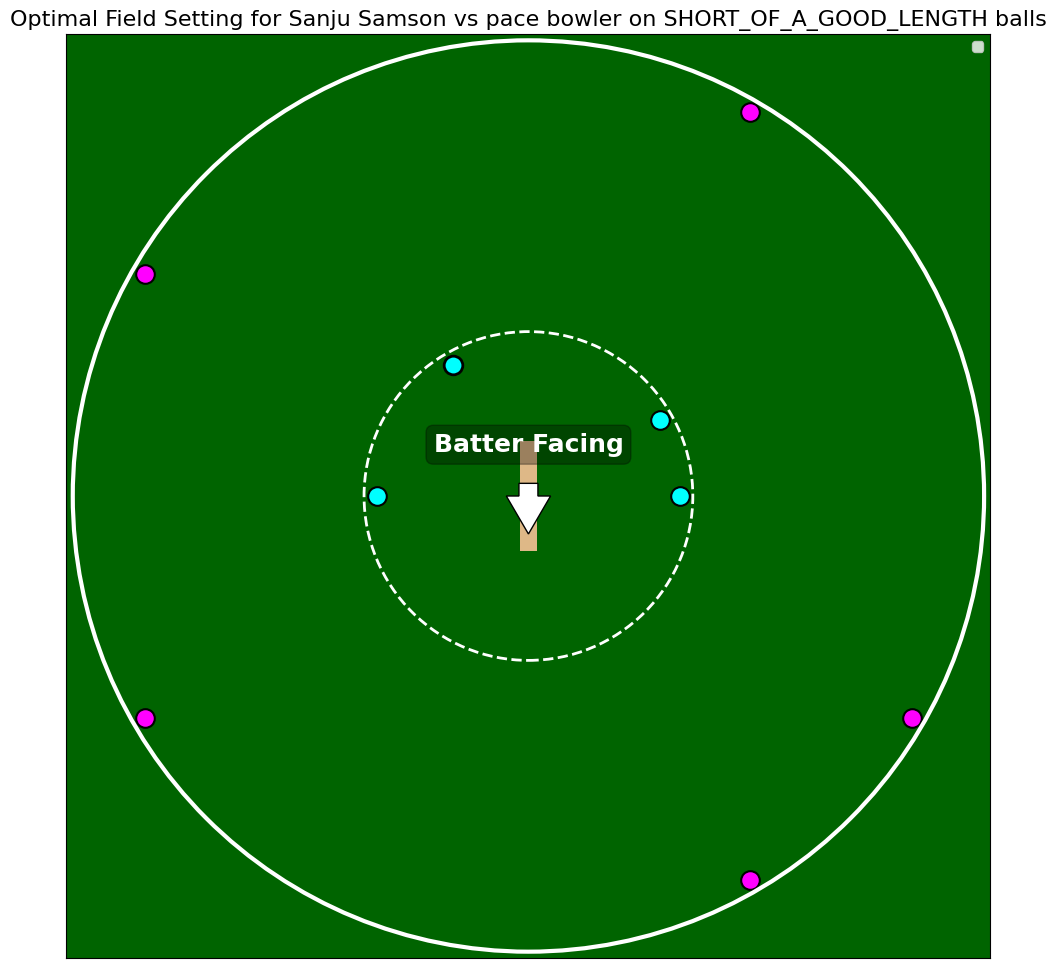
We will use the 30-degree (15 on either side) coverage area of a fielder to know how much we protect. The coverage area is placed on the field to see what sectors are covered by the fielder. The sum of expected runs (running class for an infielder, boundary class for an outfielder) of each covered sector is the total expected runs saved by the fielder (there might be some fractionally covered sectors; I have multiplied the contribution of those sectors by the respective fraction). These are the protection metrics for Sanju’s field:

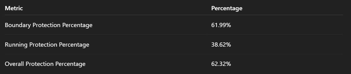
Samson on short of good is an underrated player of the cut shot. His efficiency of finding gaps when he jumps and cuts these deliveries is impressive. While the fielder waiting at deep mid wicket for the pull still covers his highest boundary percentage (20.57% boundary class coverage) being a six dominant region, the second highest boundary coverage is of the deep back point (18.86%). Following the same trend, a short third man position is effective against him as it covers 19.2% of his running class runs - the most among all infielders. I have also provided a link at the end where you can see this for different batters with individual fielder contributions.

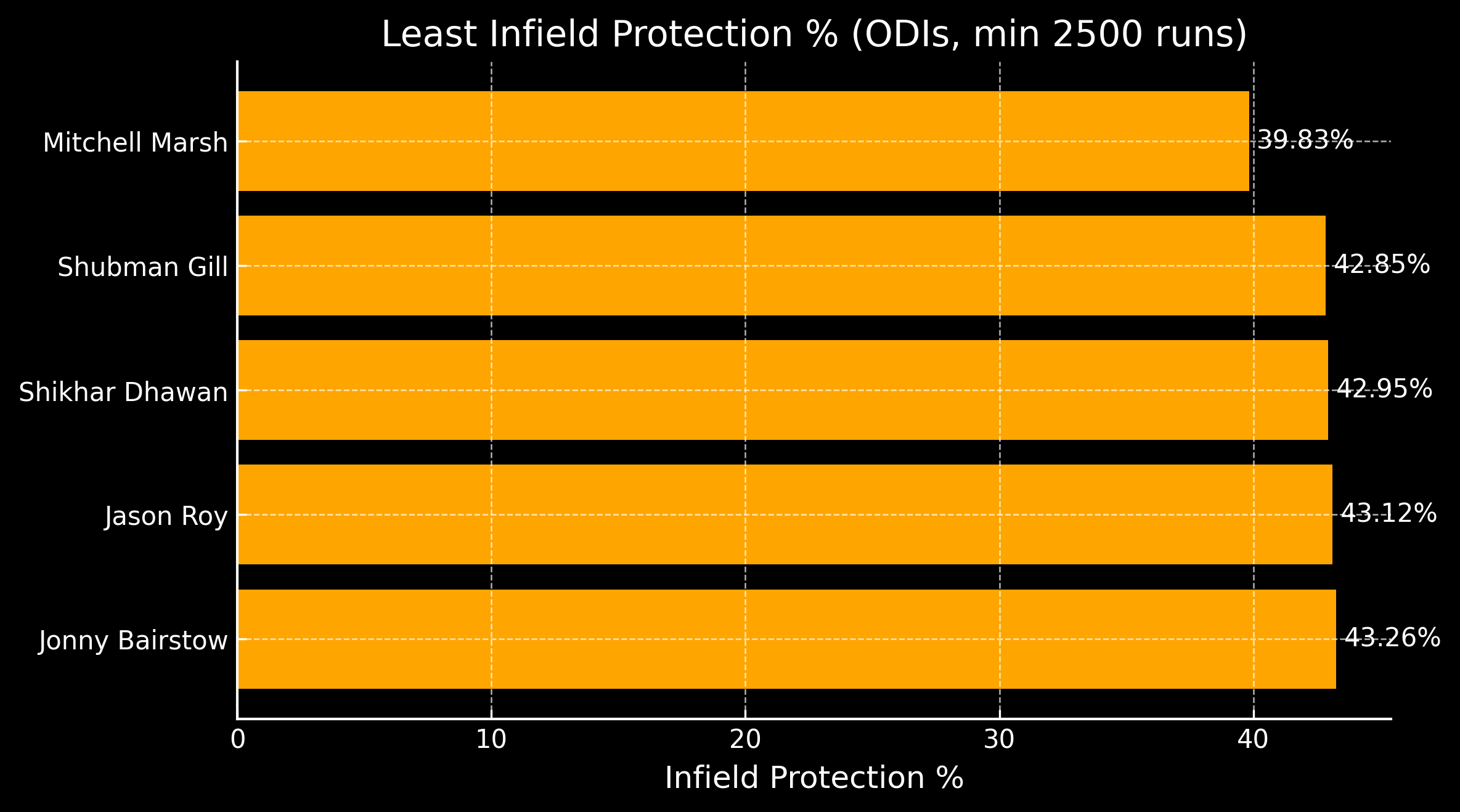
Another reason why Gill is a phenomenal ODI batter

Everyone pretty much agrees that Gill is the most ‘in-control’ white-ball batter in the game today. When we combine these control statistics with the fact that he can cut through the infield for singles at will, we see a batter on the path to becoming an all-time ODI great (if the format survives). Gill’s optimal ODI field setting (in overs 11-40) can only stop 42.85% of his infield game—the second-lowest percentage among batters with a minimum of 2,500 runs.

This ability also helped him in the IPL this year. What allowed Sai Sudharsan and Gill to score at 10 runs per over with ease was their knack for taking four to five singles every over, combined with the consistent boundaries. An approach like this can only work in T20s if the dot percentage is extremely low, and this is true for Gill because he avoids infield fielders on most occasions.

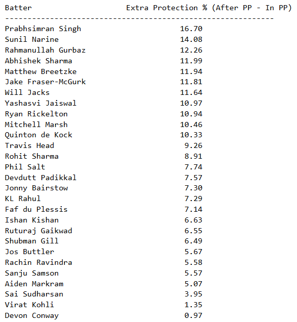
Overall Protection and Powerplay

The protection metrics help quantify the effect of fielding restrictions in the Powerplay. We analyze the difference between the Overall Protection Percentage with five outfielders versus two outfielders for openers who have played in the IPL this year. The results reinforce the idea of having boundary hitters in the Powerplay because of the low protection they have to deal with for their game. A batter with a high running class percentage won't benefit much from the field restrictions. We see this in the low "extra protection" that fielding sides get against batters like Conway and Kohli once the Powerplay is over. Aggressive batters tend to get an average 10% boost from facing less protection in the Powerplay. This explains why a Narine at the top was a progressive move at the time.

Calculated vs pace

Special Fielders

The individual run-saving numbers for each fielder help us in taking a set of crucial decisions - which fielders to place where? I’ll try explaining it with a few examples. Lets have a set of three special fielders at our disposal - the 30-Yard Wall (max protection inside 30-yards), The Sprinter (excellent in charging and throwing), The Catcher (best catching efficiency). The 30-Yard Wall is the best infielder, placed at position expected to save maximum running class runs. The Catcher is at best boundary class saving position in the outfield. We use the Sprinter to cover somewhat for our assumption of boundary fielders not saving ones, twos and threes. Sprinter is an outfielder with highest running class runs in his covered sectors.

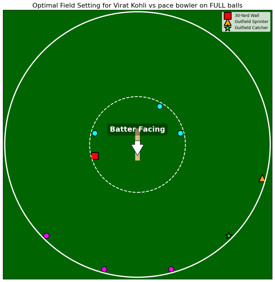
Kohli against full pace deliveries has two different shots in similar regions yielding contrasting results. A flick towards mid-wicket for running, slog towards cow corner for boundaries.

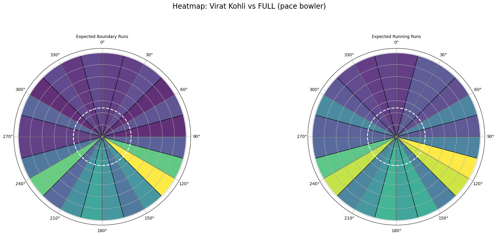
This makes us use a Sprinter and a Catcher effectively when he’s batting. In the infield, the fielder at cover needs to be the wall, holding guard against his cover drives.

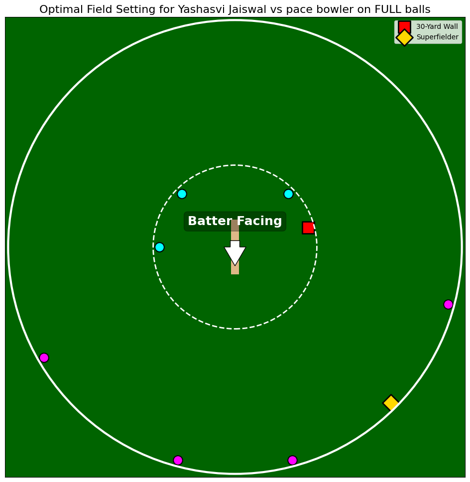
Okay, I’ll provide you with some more freedom - you can also trade a sprinter plus catcher for a Superfielder (having characteristics of both sprinter and catcher). These are cases where highest boundary class outfield position coincides with highest running class outfield position.

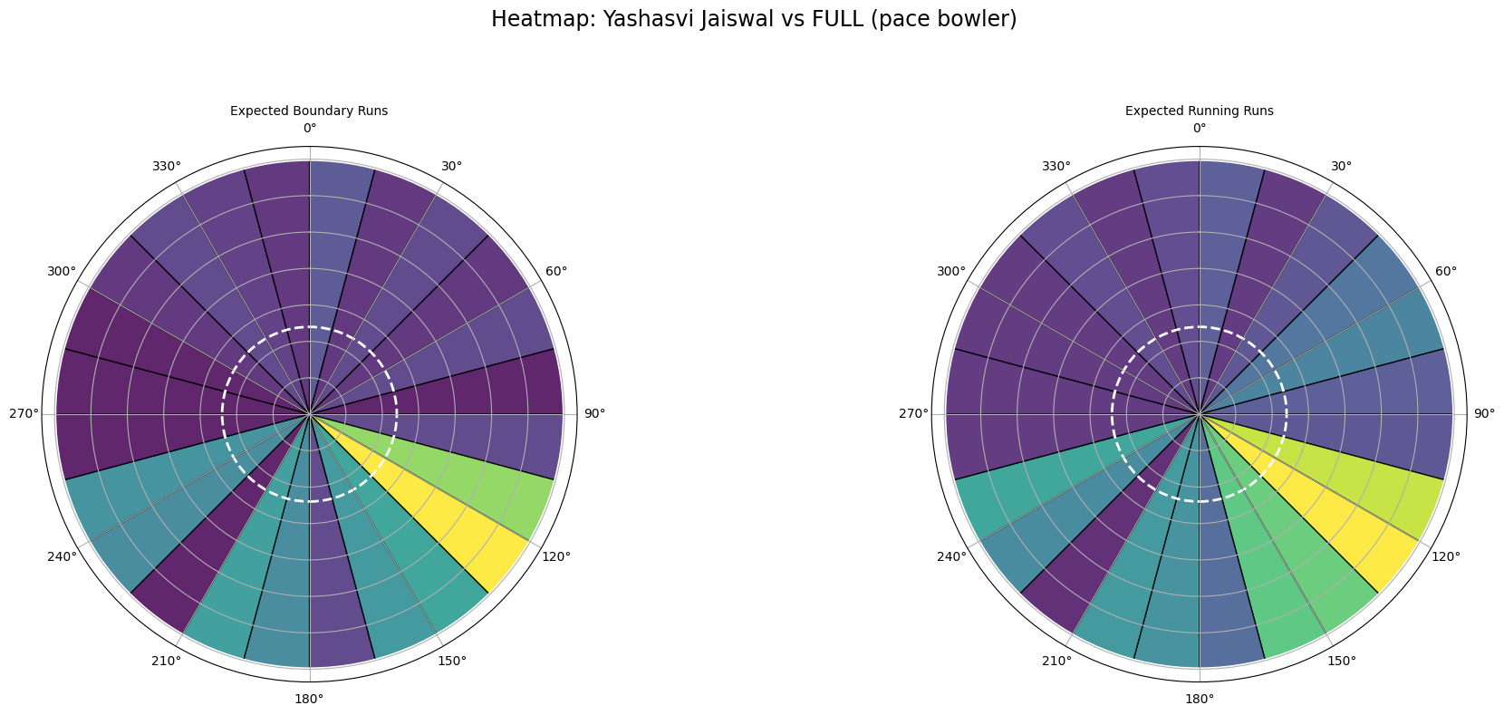
This happens for example when Jaiswal is provided with a full delivery. With an ability to drive along the ground as well as smoke flat sixes over covers, it becomes a hot zone for the fielding sides to take care of. This region as the algorithm suggests should be covered by a Superfielder.

The recognition of special fielders again requires fielding data. It’s pretty straightforward to find out exact field positions with fielder names by feeding the current setup with fielder information, once this data becomes a reality.

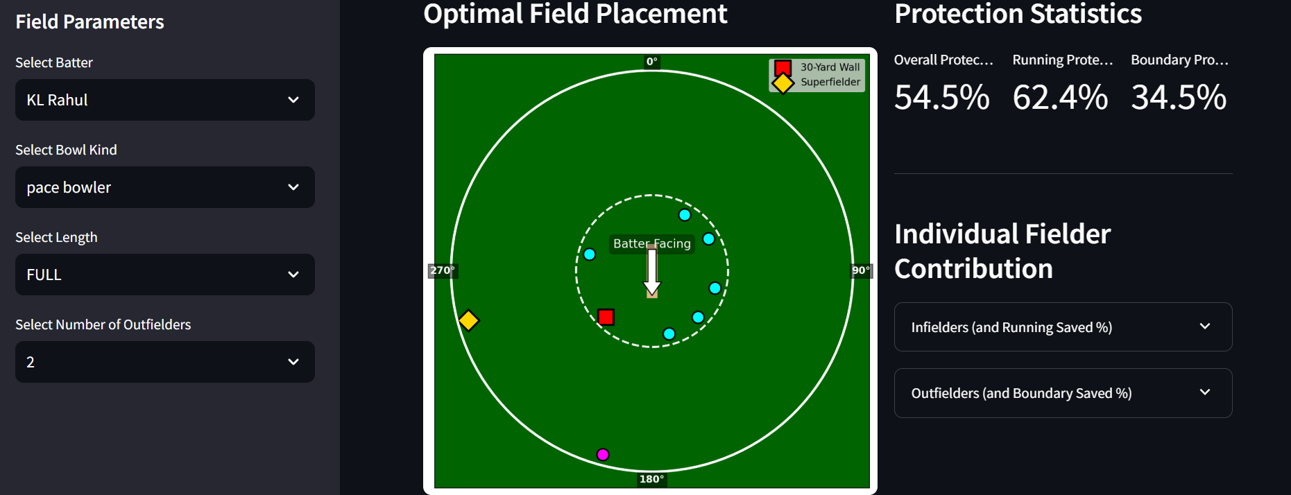
Try it yourself

This is a link (laptops/tablets screens preferred) where you can check optimal field settings.

Some Insights Using the Optimal Field Algorithm

Boundary Protection and 360 Degree Play

An Animation: Illustrating the Algorithm at work

Developing sweeps vs full length spin deliveries

I’ll end it here, hoping you liked what you read. Do share and subscribe!